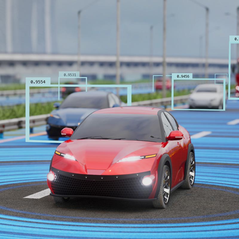
Design AI Models and AI-Driven Systems

Virtual, in-person, and self-paced courses accommodate various learning styles and organizational needs.
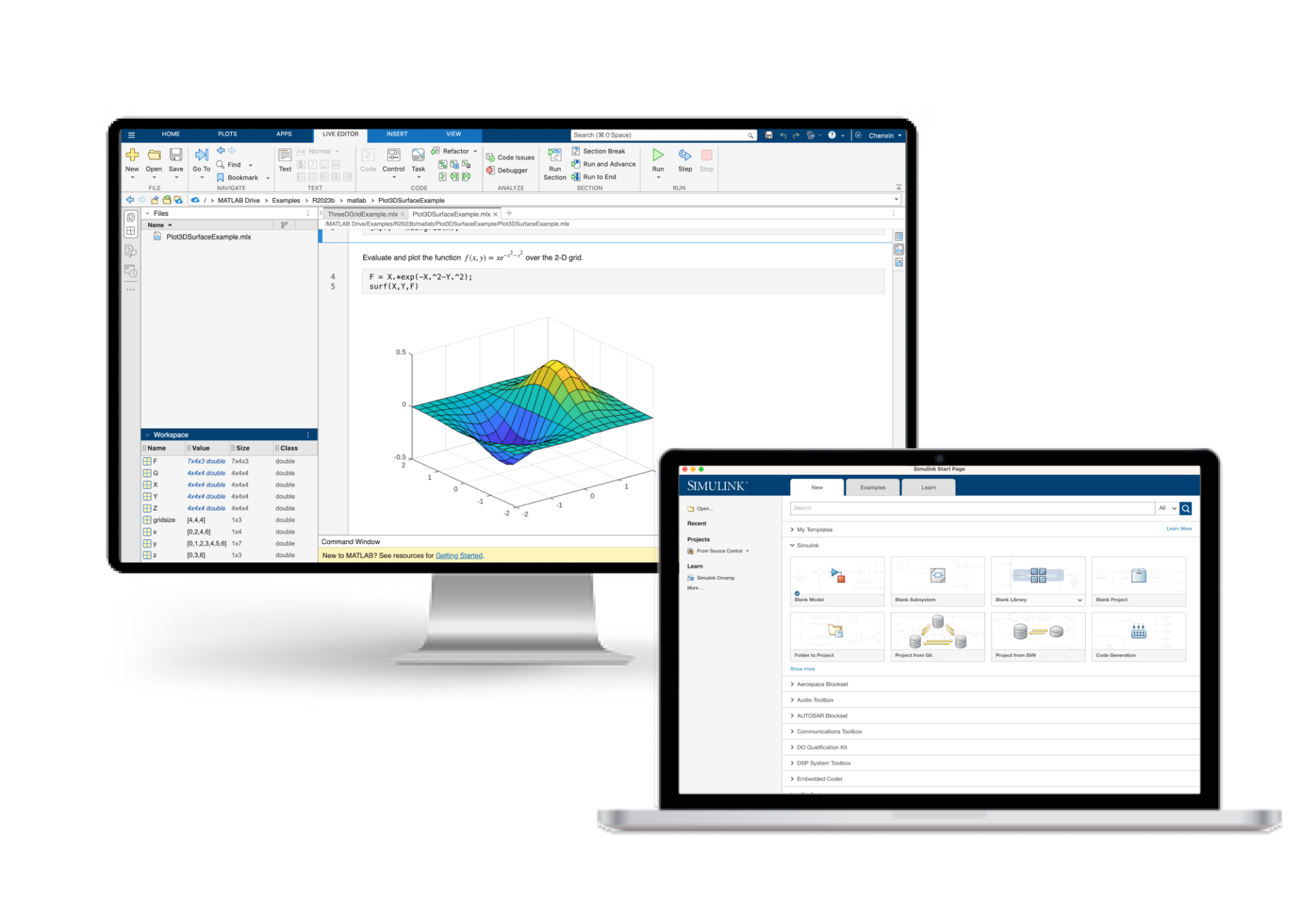
Learn core MATLAB functionality for data analysis, modeling, and programming.
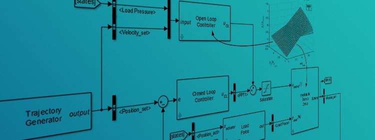
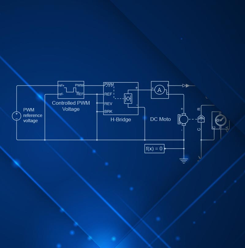
Discover dynamic system modeling, model hierarchy, and component reusability in this comprehensive introduction to Simulink.

Find project ideas, courseware, and tools to enhance your curriculum.

Discover student competitions, training resources, and more for learning with MATLAB and Simulink.
Have questions? Contact sales.
You can also select a web site from the following list
Americas
Europe
Asia Pacific